Confidence Intervals
Chapter 10
(Part 2)

Why do we need CIs?

Reporting a range of values via a confidence interval takes into account the uncertainty (sampling variation) associated with the fact that we are observing a single random sample.

We know a sampling distribution (thousands of replicate samples) center around the population parameter.
We don’t know the true value of the population parameter.
We know a sampling distribution is normally distributed (CLT)
We have no idea where our single sample falls in the sampling distribution (close to the population parameter or far away).

Check your understanding

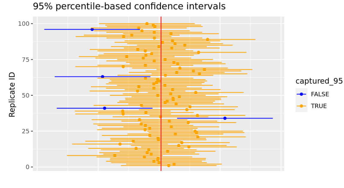
When we use a \(95\%\) critical value, approximately \(95\%\) of the confidence intervals contain the true population parameter (e.g. \(\mu\), \(\mu_1 - \mu_2\), \(\pi\), etc).

Say we generate 20,000 sample means and construct a 95% CI for each sample. How many of the constructed confidence intervals do you expect to contain the true population mean?

Width of an Interval (Margin of Error)

\[\mathbf{\hbox{Margin of Error}} = \hbox{Critical Value} * SE(\hbox{Estimator})\]

There is a trade-off between the width of an interval and the level of confidence (critical value).

Using a lower CI (ex: 90% vs 95%) decreases the margin of error (narrower interval), but a narrower CI increase the chance that your interval will not capture the true mean.
A 99% CI has a higher chance of capturing the true mean than a 95% CI, but it might be too wide of an interval to be practically useful.
You can also decrease the margin of error by increasing sample size.

Example

Let’s consider our example from last lecture. You are interested in the average weight of penguins in Antarctica. Let’s say we are able to obtain a random sample of penguins in Antarctica (for example purposes this random sample will be the penguins dataset from the palmerpenguins package.)

Baseline
Lower CI
Smaller n

Construct a 95% confidence interval for the population mean.

t.test(penguins$body_mass_g, conf.level = 0.95)


    One Sample t-test

data:  penguins$body_mass_g
t = 96.893, df = 341, p-value < 2.2e-16
alternative hypothesis: true mean is not equal to 0
95 percent confidence interval:
 4116.458 4287.050
sample estimates:
mean of x 
 4201.754

Construct a 90% confidence interval instead.

t.test(penguins$body_mass_g, conf.level = 0.90)


    One Sample t-test

data:  penguins$body_mass_g
t = 96.893, df = 341, p-value < 2.2e-16
alternative hypothesis: true mean is not equal to 0
90 percent confidence interval:
 4130.231 4273.277
sample estimates:
mean of x 
 4201.754

What if we only had a sample size of 50? Construct a 95% confidence interval.

penguins_sample <- penguins %>% 
  sample_n(size = 50)

t.test(penguins_sample$body_mass_g, conf.level = 0.95)


    One Sample t-test

data:  penguins_sample$body_mass_g
t = 39.648, df = 49, p-value < 2.2e-16
alternative hypothesis: true mean is not equal to 0
95 percent confidence interval:
 3843.777 4254.223
sample estimates:
mean of x 
     4049

Extra practice

We are interested in making inferences about penguins that live near Palmer Station, Antarctica. We will use the penguins data from the palmerpenguins package as our “random” sample.

library(palmerpenguins)

# type data(penguins) in console for dataset to appear in environment

Construct a 90% CI for the difference in average flipper length between the Adelie penguins and the Gentoo.
Construct a 97% CI for the proportion of penguins that are of the Gentoo species.
Construct a 99% CI for the difference in the proportion of female penguins of the Adelie or Chinstrap species that weigh over 4000 g and the proportion of male penguins of the Adelie or Chinstrap that weigh over 4000 g
Run a simple linear regression to predict body_mass_g based on flipper_length_mm. What is the 97% confidence interval for the slope?

Solutions

Construct a 90% CI for the difference in average flipper length between the Adelie penguins and the Gentoo penguins.

penguins_adelie <- penguins %>% 
  filter(species == "Adelie")

penguins_gentoo <- penguins %>% 
  filter(species == "Gentoo")

t.test(x = penguins_adelie$flipper_length_mm, 
       y = penguins_gentoo$flipper_length_mm,
       conf.level = 0.9)


    Welch Two Sample t-test

data:  penguins_adelie$flipper_length_mm and penguins_gentoo$flipper_length_mm
t = -34.445, df = 261.75, p-value < 2.2e-16
alternative hypothesis: true difference in means is not equal to 0
90 percent confidence interval:
 -28.53846 -25.92824
sample estimates:
mean of x mean of y 
 189.9536  217.1870

We are 90% confident that the difference in average flipper length of the Adelie species and Gentoo species of penguins in Palmer Station, Antarctica is between -28.54 and -25.93 mm.

(This means we are 90% confident the Adelie species flippers are between 25.93 and 28.54 mm shorter than the Gentoo species for penguins in Palmer Station, Antarctica.)

Construct a 97% CI for the proportion of penguins that are of the Gentoo species.

we want the count of Gentoo and count of penguins sampled
count of penguins sampled can be seen by looking at num obs in environment OR add up all the counts (152 + 68 + 124)

# Option 1
# use count and pick out correct number
penguins |> 
  count(species)

# A tibble: 3 × 2
  species       n
  <fct>     <int>
1 Adelie      152
2 Chinstrap    68
3 Gentoo      124

# Option 2
# use filter to get count
penguins %>% 
  filter(species == "Gentoo") |> 
  summarize(n = n())

# A tibble: 1 × 1
      n
  <int>
1   124

prop.test(x = 124, n = 344,
          conf.level = 0.97)


    1-sample proportions test with continuity correction

data:  124 out of 344, null probability 0.5
X-squared = 26.235, df = 1, p-value = 3.022e-07
alternative hypothesis: true p is not equal to 0.5
97 percent confidence interval:
 0.3051357 0.4196602
sample estimates:
        p 
0.3604651

We are 97% confident that the proportion of penguins in Palmer Station, Antarctica that are Gentoo is between 0.3051 and 0.4197.

Construct a 99% CI for the difference in the proportion of female penguins of the Adelie or Chinstrap species that weigh over 4000 g and the proportion of male penguins of the Adelie or Chinstrap that weigh over 4000 g

we are sampling “female” and “male penguins those are my 2 denominators!
numerator 1 = female & (Adelie or Chinstrap) & over 4000 g
numerator 2 = male & (Adelie or Chinstrap) & over 4000 g

# get my denominators n = c(#, #)
penguins %>%
  count(sex)

# A tibble: 3 × 2
  sex        n
  <fct>  <int>
1 female   165
2 male     168
3 <NA>      11

# get my numerators of interest
peng_new <- penguins %>% 
  filter(species != "Gentoo", body_mass_g > 4000)
# ALTERNATE way to filter
# filter(species == "Adelie" | species == "Chinstrap", body_mass_g > 4000)

# check dataset in environment to make sure it looks correct
peng_new |> 
  count(sex)

# A tibble: 3 × 2
  sex        n
  <fct>  <int>
1 female     1
2 male      48
3 <NA>       1

prop.test(x = c(1, 48), n = c(165, 168),
          conf.level = 0.99)


    2-sample test for equality of proportions with continuity correction

data:  c(1, 48) out of c(165, 168)
X-squared = 49.671, df = 1, p-value = 1.818e-12
alternative hypothesis: two.sided
99 percent confidence interval:
 -0.3767761 -0.1825313
sample estimates:
     prop 1      prop 2 
0.006060606 0.285714286

We are 99% confident that the difference in proportion of penguins in Palmer Station, Antarctica that are female of the Adelie or Chinstrap species that weigh over 4000 g and the proportion of male of the Adelie or Chinstrap that weigh over 4000 g is between -0.3768 and -0.1825.

Run a simple linear regression to predict body_mass_g based on flipper_length_mm. What is the 97% confidence interval for the slope?

model_peng <- lm(body_mass_g ~ flipper_length_mm, data = penguins)

confint(model_peng, level = 0.97)

                       1.5 %      98.5 %
(Intercept)       -6447.2738 -5114.38891
flipper_length_mm    46.3766    52.99453

We are 97% confident that for every 1mm increase in flipper length, a penguins body mass is expected to increase somewhere between 46.38 and 52.99 grams.