P-values
Chapter 11

Overview

We have a claim about a population parameter and form competing hypothesis to test the claim.
We then determine which hypothesis is better supported by our sample data.
We are always forming the hypothesis about a population parameter.

Hypothesis test

$H_0$ (Null Hypothesis): The population parameter is a particular value and any observed sample differences is due to chance variation. This is what we expect.

$H_A$ (Alternative Hypothesis): There is a reason besides chance that explains the sample data.

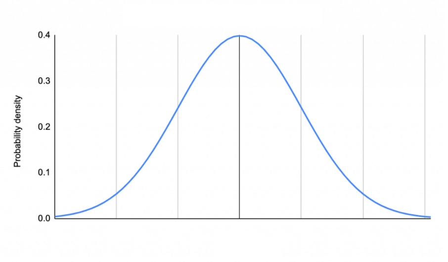
Writing hypotheses examples (two-sided)

$H_0$: $\mu=5$

$H_A$: $\mu\ne5$

$H_0$: $\pi=0.5$

$H_A$: $\pi\ne0.5$

$H_0$: $\mu_1-\mu_2=0$

$H_A$: $\mu_1-\mu_2\ne0$

$H_0$: $\beta_1=0$

$H_A$: $\beta_1\ne0$

These are called two-sided tests. There also exists one-sided tests ex: $H_0: \pi = 0.5$ vs $H_A: \pi < 0.5$ but should generally not be used unless you have a very strong reason to only be interested in the effect occurring in one specific direction, and are completely unconcerned about the possibility of an effect in the opposite direction.

Writing hypotheses examples (One-sided)

$H_0$: $\mu=5$

$H_A$: $\mu>5$

$H_0$: $\pi=0.5$

$H_A$: $\pi<0.5$

$H_0$: $\mu_1-\mu_2=0$

$H_A$: $\mu_1-\mu_2>0$

$H_0$: $\beta_1=0$

$H_A$: $\beta_1<0$

These are called one-sided tests.

Potential pitfalls of one-sided tests

Data fishing: If you choose the direction of the one-sided test after looking at the data, it can lead to misleading results.
Missing important information: If a significant effect occurs in the “wrong” direction, a one-sided test might miss it completely.
Use them only if you are certain about that there is only one possible direction of values for the random variable, before conducting the test.

P-values

In order to determine if the null hypothesis is likely to be true we calculate a p-value.
p-value: probability of observing an estimate as extreme as the one you observed from the data if the null was true.
A small p-value means the observed sample data is unlikely to occur under the null hypothesis. ie: proof by contradiction. Reject the null hypothesis because it is probably not true.

One-sample (two-sided) tests

Statistic	$H_0$	$H_A$	Test Statistic (STAT)	Distribution
Mean	$\mu= \mu_0$	$\mu \neq \mu_0$	$\frac{\bar{x} - \mu_0}{s/\sqrt{n}}$	t(df=n-1)
Proportion	$\pi = \pi_0$	$\pi \neq \pi_0$	$\frac{\hat{\pi}-\pi_0}{\sqrt{\frac{\pi_0(1-\pi_0)}{n} } }$	N(0,1)

Two-sample (two-sided) tests

For two-sample tests there are 2 ways to calculate the SE

Assume the two samples have the same variance and use a pooled (equal variance) formula
Assume the two samples have unequal variances and use an unpooled (unequal variance) formula

Two-sided tests for Pooled (equal) Variances

Statistic	$H_0$	$H_A$	Test Statistic	Distribution
Diff. in means	$\mu_1-\mu_2 = d$	$\mu_1-\mu_2 \neq d$	$\frac{\bar{x_1} - \bar{x_2}-d}{s_p\sqrt{\frac{1}{n_1}+\frac{1}{n_2}}}$	$t(df=n_1 + n_2 -2)$
Diff. in proportions	$\pi_1-\pi_2 = 0$	$\pi_1-\pi_2 \neq 0$	$\frac{(\hat{\pi_1}-\hat{\pi_2}) - 0}{\sqrt{\frac{\hat{\pi_0}(1-\hat{\pi_0})}{n_1} + \frac{\hat{\pi_0}(1-\hat{\pi_0})}{n_2} } }$	$N(0,1)$

Two-sided tests for Unpooled (unequal) Variances

Statistic	$H_0$	$H_A$	Test Statistic	Distribution
Diff. in means	$\mu_1-\mu_2 = d$	$\mu_1-\mu_2 \neq d$	$\frac{\bar{x_1}-\bar{x_2}-d}{\sqrt{\frac{s_1^2}{n_1}+\frac{s_2^2}{n_2}}}$	$t(df=min(n_1-1, n_2-1) )$
Diff. in proportions	$\pi_1-\pi_2 = d$	$\pi_1-\pi_2 \neq d$	$\frac{(\hat{\pi_1}-\hat{\pi_2}) - d}{\sqrt{\frac{\hat{\pi_1}(1-\hat{\pi_1})}{n_1} + \frac{\hat{\pi_2}(1-\hat{\pi_2})}{n_2} } }$	$N(0,1)$

R Code to obtain p-value

Statistic	R Code
Mean	t.test(x = data$variable, mu = $\mu_0$)
Proportion	prop.test(x = #, n = #, p= $\pi_0$, correct=FALSE)
Regression slope	lm() summary
Diff in mean	t.test(x = data1$variable, y = data2$variable)
Diff in proportion	prop.test(x = c(#, #), n = c(#, #), correct=FALSE )

Example 1

You heard a zoologist claim the average weight of penguins is at least 4250 g.

You want to test this claim so you collect a random sample of penguins and measure their weight, stored in the penguins dataset from the palmerpenguins package.

What is the null and alternative hypothesis?

\[H_0: \pi_{weight} = 4250\] \[H_A: \pi_{weight} \ne 4250\]
\[H_0: \mu_{weight} > 4250\] \[H_A: \mu_{weight} \leq 4250\]
\[H_0: \bar{x}_{weight} = 4250\] \[H_A: \bar{x}_{weight} \ne 4250\]

\[H_0: \mu_{weight} = 4250\] \[H_A: \mu_{weight} \ne 4250\]
\[H_0: \bar{x}_{weight} \geq 4250\] \[H_A: \bar{x}_{weight} < 4250\]

Example 1

You heard a zoologist claim the average weight of penguins is at least 4250 g.

You want to test this claim so you collect a random sample of penguins and measure their weight, stored in the penguins dataset from the palmerpenguins package.

$H_0:$

$H_A:$

t.test(x = penguins$body_mass_g, mu = 4250)


    One Sample t-test

data:  penguins$body_mass_g
t = -1.1126, df = 341, p-value = 0.2667
alternative hypothesis: true mean is not equal to 4250
95 percent confidence interval:
 4116.458 4287.050
sample estimates:
mean of x 
 4201.754

Example 2

You think that 33% of penguins belong to the Adelie species.

You want to test this claim so you collect a random sample of penguins and count how many are of the Adelie species, stored in the penguins dataset from the palmerpenguins package.

$H_0:$

$H_A:$

penguins %>% 
  count(species)

# A tibble: 3 × 2
  species       n
  <fct>     <int>
1 Adelie      152
2 Chinstrap    68
3 Gentoo      124

prop.test(x = 153, n = 344, p = 0.33)


    1-sample proportions test with continuity correction

data:  153 out of 344, null probability 0.33
X-squared = 19.977, df = 1, p-value = 7.837e-06
alternative hypothesis: true p is not equal to 0.33
95 percent confidence interval:
 0.3917305 0.4990579
sample estimates:
        p 
0.4447674

Statistic	\(H_0\)	\(H_A\)	Test Statistic (STAT)	Distribution
Mean	\(\mu= \mu_0\)	\(\mu \neq \mu_0\)	\(\frac{\bar{x} - \mu_0}{s/\sqrt{n}}\)	t(df=n-1)
Proportion	\(\pi = \pi_0\)	\(\pi \neq \pi_0\)	\(\frac{\hat{\pi}-\pi_0}{\sqrt{\frac{\pi_0(1-\pi_0)}{n} } }\)	N(0,1)

Statistic	\(H_0\)	\(H_A\)	Test Statistic	Distribution
Diff. in means	\(\mu_1-\mu_2 = d\)	\(\mu_1-\mu_2 \neq d\)	\(\frac{\bar{x_1} - \bar{x_2}-d}{s_p\sqrt{\frac{1}{n_1}+\frac{1}{n_2}}}\)	\(t(df=n_1 + n_2 -2)\)
Diff. in proportions	\(\pi_1-\pi_2 = 0\)	\(\pi_1-\pi_2 \neq 0\)	\(\frac{(\hat{\pi_1}-\hat{\pi_2}) - 0}{\sqrt{\frac{\hat{\pi_0}(1-\hat{\pi_0})}{n_1} + \frac{\hat{\pi_0}(1-\hat{\pi_0})}{n_2} } }\)	\(N(0,1)\)

Statistic	\(H_0\)	\(H_A\)	Test Statistic	Distribution
Diff. in means	\(\mu_1-\mu_2 = d\)	\(\mu_1-\mu_2 \neq d\)	\(\frac{\bar{x_1}-\bar{x_2}-d}{\sqrt{\frac{s_1^2}{n_1}+\frac{s_2^2}{n_2}}}\)	\(t(df=min(n_1-1, n_2-1) )\)
Diff. in proportions	\(\pi_1-\pi_2 = d\)	\(\pi_1-\pi_2 \neq d\)	\(\frac{(\hat{\pi_1}-\hat{\pi_2}) - d}{\sqrt{\frac{\hat{\pi_1}(1-\hat{\pi_1})}{n_1} + \frac{\hat{\pi_2}(1-\hat{\pi_2})}{n_2} } }\)	\(N(0,1)\)

Statistic	R Code
Mean	t.test(x = data$variable, mu = \(\mu_0\))
Proportion	prop.test(x = #, n = #, p= \(\pi_0\), correct=FALSE)
Regression slope	lm() summary
Diff in mean	t.test(x = data1$variable, y = data2$variable)
Diff in proportion	prop.test(x = c(#, #), n = c(#, #), correct=FALSE )

P-values Chapter 11

Overview

Hypothesis test

Writing hypotheses examples (two-sided)

Writing hypotheses examples (One-sided)

Potential pitfalls of one-sided tests

P-values

One-sample (two-sided) tests

Two-sample (two-sided) tests

Two-sided tests for Pooled (equal) Variances

Two-sided tests for Unpooled (unequal) Variances

R Code to obtain p-value

Example 1

Example 1

Example 2

P-values
Chapter 11