4  Multiple factors

4.1 Randomized complete block design (RCBD)

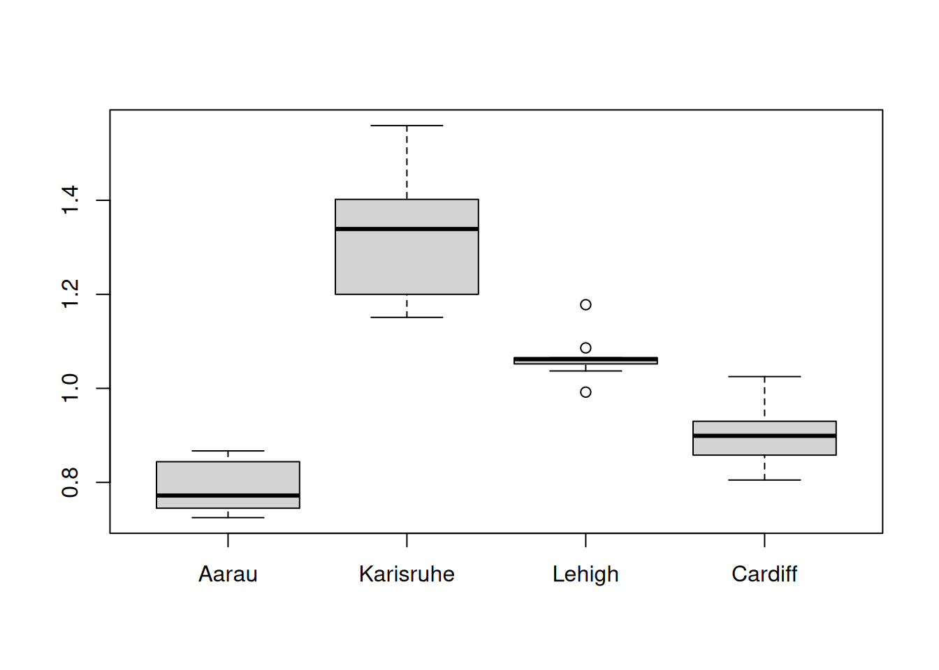
Let us consider an example, where the shear strength of steel plate girders needs to be modeled as a function of the four methods (treatment) and nine girders (blocks).

library(ACSWR)
library(reshape2)
library(DescTools)
library(lmtest)

# Visualizing treatment effects
data("girder")
boxplot(girder[,2:5])

# Melting data to make it suitable to fit a linear regression model
# using the 'lm' function
data_melt <- melt(girder, variable.name = "treatment", id = 'Girder')
anova(lm(value~Girder+treatment, data = data_melt))
Analysis of Variance Table

Response: value
          Df  Sum Sq Mean Sq F value    Pr(>F)    
Girder     8 0.08949 0.01119  1.6189    0.1717    
treatment  3 1.51381 0.50460 73.0267 3.296e-12 ***
Residuals 24 0.16584 0.00691                      
---
Signif. codes:  0 '***' 0.001 '**' 0.01 '*' 0.05 '.' 0.1 ' ' 1

The null hypothesis that there is no effect of the method on the sheer strength of the girder is rejected.

Let us compare the methods pairwise.

aov_object <- aov(value~Girder+treatment, data = data_melt)

# Tukey's method
PostHocTest(aov_object, method = "hsd")$treatment
                        diff       lwr.ci      upr.ci         pval
Karisruhe-Aarau    0.5452222  0.437124171  0.65332027 3.225975e-12
Lehigh-Aarau       0.2713333  0.163235283  0.37943138 2.106339e-06
Cardiff-Aarau      0.1106667  0.002568616  0.21876472 4.343575e-02
Lehigh-Karisruhe  -0.2738889 -0.381986940 -0.16579084 1.808447e-06
Cardiff-Karisruhe -0.4345556 -0.542653606 -0.32645750 3.675706e-10
Cardiff-Lehigh    -0.1606667 -0.268764717 -0.05256862 2.164599e-03

All methods are different from each other according to Tukey’s method (at 5% significance level).

# Bonferroni's method
PostHocTest(aov_object, method = "bonferroni")$treatment
                        diff       lwr.ci      upr.ci         pval
Karisruhe-Aarau    0.5452222  0.432559601  0.65788484 3.308011e-12
Lehigh-Aarau       0.2713333  0.158670712  0.38399595 2.208198e-06
Cardiff-Aarau      0.1106667 -0.001995955  0.22332929 5.631958e-02
Lehigh-Karisruhe  -0.2738889 -0.386551510 -0.16122627 1.894578e-06
Cardiff-Karisruhe -0.4345556 -0.547218177 -0.32189293 3.770501e-10
Cardiff-Lehigh    -0.1606667 -0.273329288 -0.04800405 2.453939e-03

All methods except Aarau and Cardiff are different from each other according to Bonferroni’s method (at 5% significance level).

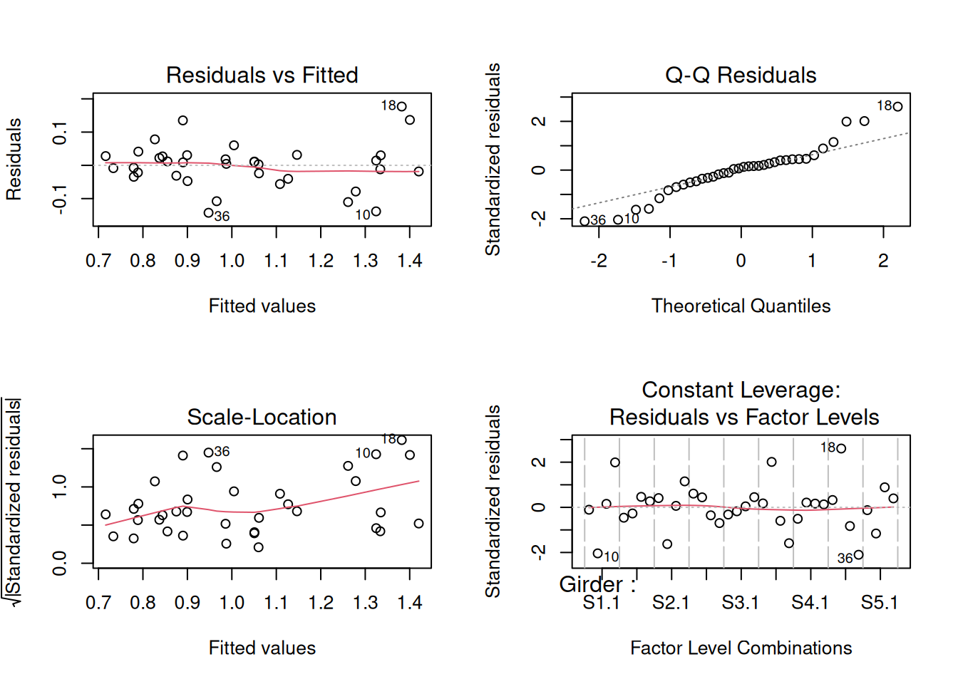
Let us verify if the model assumptions are satisfied.

par(mfrow = c(2,2))
model <- lm(value~Girder+treatment, data = data_melt)
plot(model)

shapiro.test(model$residuals)

    Shapiro-Wilk normality test

data:  model$residuals
W = 0.94966, p-value = 0.102

The errors are normally distribued.

bptest(model)

    studentized Breusch-Pagan test

data:  model
BP = 22.205, df = 11, p-value = 0.02283

The error variance assumption is also satisfied at a 1% significance level. There is no strong deviation from the assumption.

4.2 Two-way layout: Fixed effects

A manufacturer was interested in finding differences in torque values of a lock-nut. The two factors effecting the torque are the type of plating, and whether the locknut is threaded into a bolt or a mandrel. We’ll use two-way ANOVA to find if the two factors or their interaction effect the torque.

data <- read.table('bolt.dat.txt', header = TRUE)
data_melt <- melt(data, variable.name = 'plating', value.name = 'torque')
Using M.B as id variables
head(data_melt)
  M.B plating torque
1   M     P.O     10
2   M     P.O     13
3   M     P.O     17
4   M     P.O     16
5   M     P.O     15
6   M     P.O     14
anova(lm(torque ~ M.B*plating, data = data_melt))
Analysis of Variance Table

Response: torque
            Df Sum Sq Mean Sq F value    Pr(>F)    
M.B          1  821.4  821.40 22.4563 1.604e-05 ***
plating      2 2290.6 1145.32 31.3118 9.363e-10 ***
M.B:plating  2  665.1  332.55  9.0916 0.0003952 ***
Residuals   54 1975.2   36.58                      
---
Signif. codes:  0 '***' 0.001 '**' 0.01 '*' 0.05 '.' 0.1 ' ' 1
#data['plating_bolt'] = apply(data_melt[,1:2], axis = 1, function(x) paste)

The two factors and their interaction significantly effects the torque.

4.3 Two-way layout: Random effects

Ten food items are being tested by 5 judges (operators) for quality. Each judge inspects a food item 3 times, and gives a score. Answer the following questions with appropriate analysis:

  1. Is there a statistically significant variation in the scores given by judges for the same quality of food? If yes, quantify the variation.

  2. Is the variation in the scores given by judges for the same quality of food dependent on the food item?

  3. Is there a statistically significant variation in the quality of the food items after removing the variation in scores due to different judges? If yes, quantify the variation.

data <- read.csv('sensory_data.csv', header = TRUE)
head(data)
   Item Operator1 Operator2 Operator3 Operator4 Operator5
1 Item1       4.3       4.9       3.3       5.3       4.4
2 Item1       4.3       4.5       4.0       5.5       3.3
3 Item1       4.1       5.3       3.4       5.7       4.7
4 Item2       6.0       5.3       4.5       5.9       4.7
5 Item2       4.9       6.3       4.2       5.5       4.9
6 Item2       6.0       5.9       4.7       6.3       4.6
data_melt <- melt(data, variable.name = "Operator", value.name = 'property')
Using Item as id variables
head(data_melt)
   Item  Operator property
1 Item1 Operator1      4.3
2 Item1 Operator1      4.3
3 Item1 Operator1      4.1
4 Item2 Operator1      6.0
5 Item2 Operator1      4.9
6 Item2 Operator1      6.0
anova(lm(property~Item*Operator, data = data_melt))
Analysis of Variance Table

Response: property
               Df Sum Sq Mean Sq  F value    Pr(>F)    
Item            9 612.40  68.044 199.3084 < 2.2e-16 ***
Operator        4  25.49   6.372  18.6643 1.739e-11 ***
Item:Operator  36  12.97   0.360   1.0549     0.406    
Residuals     100  34.14   0.341                       
---
Signif. codes:  0 '***' 0.001 '**' 0.01 '*' 0.05 '.' 0.1 ' ' 1

Yes, there is a statistically significant variation in the scores given by judges for the same quality of food

The standard deviation in the scores given by judges for the same quality of food is:

sqrt((6.37 - 0.36)/30)
[1] 0.4475861

The variation in the scores given by judges for the same quality of food does not depend on the food item

Yes, there is a statistically significant variation in the quality of the food items after removing the variation in scores due to different judges.

The standard deviation in the scores given food items after removing the variation due to different judges is:

sqrt((68.04 - 0.36)/15)
[1] 2.124147