library(maximin)6 Computer experiment designs
6.1 Maximin design
Let us generate a 4-run maximin design in \([0, 1]^2\) for \(p=2\).
We will use the maximin() function of the maximin library
For generating a maximin design, we need to specify an initial design, and the function will add points to the design to develop a design that is as close to a maximin design as possible.
Let us add the origin as a point in the initial design.
D_initial <- matrix(c(0,0),1,2)set.seed(3)
D <- maximin(n = 3, p=2, Xorig = D_initial)$Xfpar(pty="s") # Making a square plot (maintaining aspect ratio)
plot(D, pch = 16)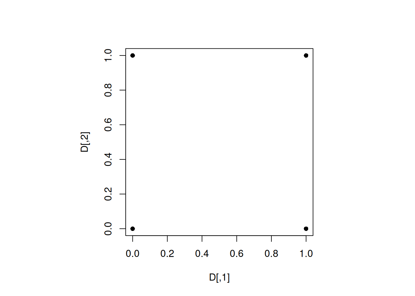
As expected, the design is the four corners of the feasible design space as the minimum distance between any two design points is the largest in this case.
Note that the algorithm that maximizes the minimum distance between points is an iterative algorithm that does not guarantee to find the global optimum. The more iterations it runs, the higher is the likelihood to find the global optimum. One can increase the number of iterations of the optimization algorithm, and / or execute the code multiple times, and compare the minimum distance between points to obtain a better maximin design.
Let us attempt to obtain a 5-run maximin design in \([0, 1]^2\) for \(p=2\).
set.seed(3)
D <- maximin(n = 4, p=2, Xorig = D_initial)
par(pty="s")
plot(D$Xf, pch = 16)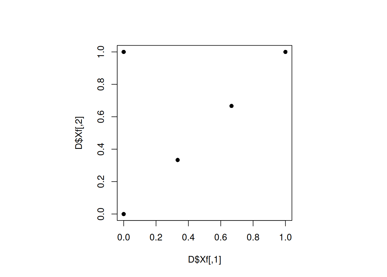
Let us compute the maximin distance for this design.
# Function to obtain the minimum distance between
# a point and a design
minimum_distance <- function(x, D)
{
  sq_distances <- (colSums((t(D)- x)^2))
  sq_distances[sq_distances == 0] <- Inf
  return(sqrt(min(sq_distances)))
}
min(apply(D$Xf, 1, minimum_distance, D = D$Xf))
[1] 0.4713757Let us increase the iterations of the maximin() function to see if that leads to a better design.
set.seed(3)
D <- maximin(n = 4, p=2, Xorig = D_initial, T = 100)
par(pty="s")
plot(D$Xf, pch = 16)
min(apply(D$Xf, 1, minimum_distance, D = D$Xf))[1] 0.4714045Increasing the number of iteration did not help. We can increase the iterations further. However, let us try to change the seed.
set.seed(4)
D <- maximin(n = 4, p=2, Xorig = D_initial, T = 100)
par(pty="s")
plot(D$Xf, pch = 16)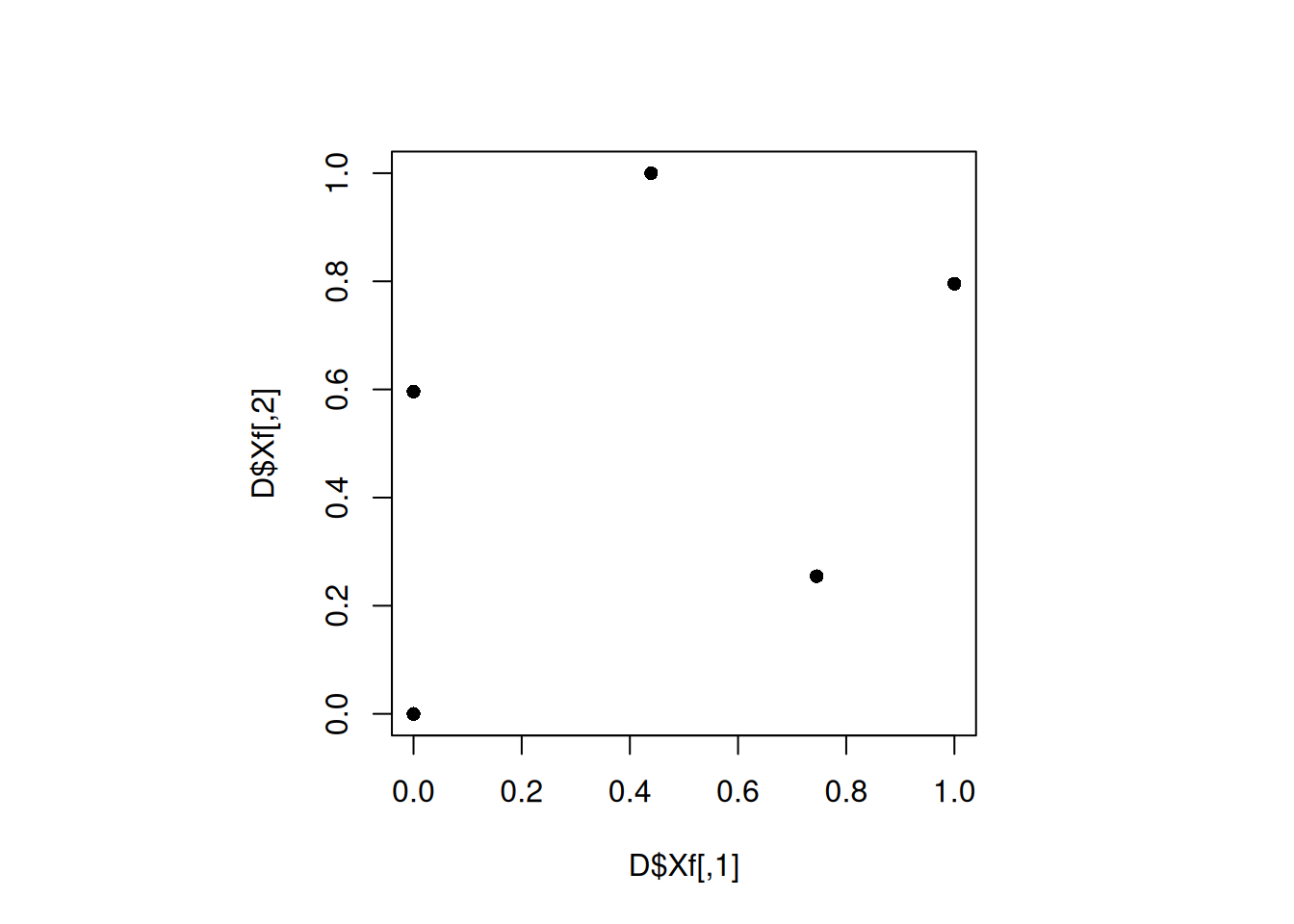
min(apply(D$Xf, 1, minimum_distance, D = D$Xf))[1] 0.5962154We got a better design, as the minimum distance between the points is higher. Let us increase the number of iterations to see if the design gets better.
set.seed(4)
D <- maximin(n = 4, p=2, Xorig = D_initial, T = 200)
par(pty="s")
plot(D$Xf, pch = 16)
min(apply(D$Xf, 1, minimum_distance, D = D$Xf))[1] 0.6469957The design gets better with increased iterations. Let us further increase the iterations.
set.seed(4)
D <- maximin(n = 4, p=2, Xorig = D_initial, T = 400)
par(pty="s")
plot(D$Xf, pch = 16)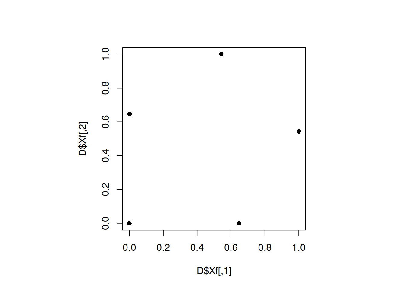
min(apply(D$Xf, 1, minimum_distance, D = D$Xf))[1] 0.6468853The design did not get better. Let us change the seed again.
set.seed(5)
D <- maximin(n = 4, p=2, Xorig = D_initial, T = 400)
par(pty="s")
plot(D$Xf, pch = 16)
min(apply(D$Xf, 1, minimum_distance, D = D$Xf))[1] 0.4714045The design did not get better. Let us change use a for() loop to try a lot of different seeds.
min_dist <- rep(0, 20)
for(s in 1:20)
{
  set.seed(s)
  D <- maximin(n = 4, p=2, Xorig = D_initial, T = 100)
  min_dist[s] <- min(apply(D$Xf, 1, minimum_distance, D = D$Xf))
}
The seed for the best design, i.e., the design with the maximum minimum distance between points is:
which.max(min_dist)[1] 12Let us plot the best design:
set.seed(12)
D <- maximin(n = 4, p=2, Xorig = D_initial, T = 100)
par(pty="s")
plot(D$Xf, pch = 16)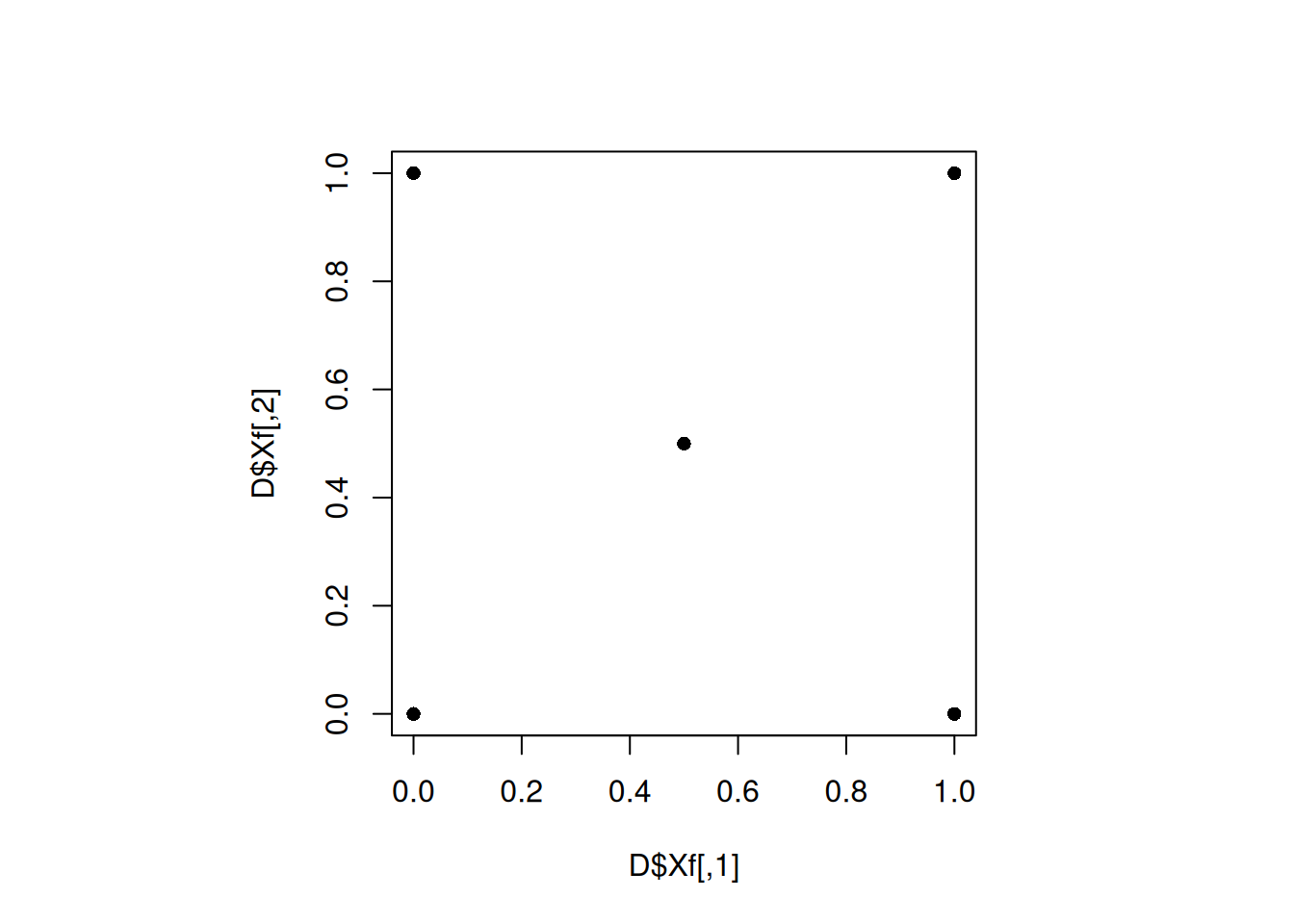
min(apply(D$Xf, 1, minimum_distance, D = D$Xf))[1] 0.70710686.2 Maximin LHD
Let us generate a 4-run maximin LHD in \([0, 1]^2\) for \(p=2\).
We will use the maximinLHS() function of the lhs library
library(lhs)set.seed(1)
D <- maximinLHS(4, 2)
par(pty="s")
plot(D, xlim = c(0, 1), ylim = c(0, 1), pch = 16)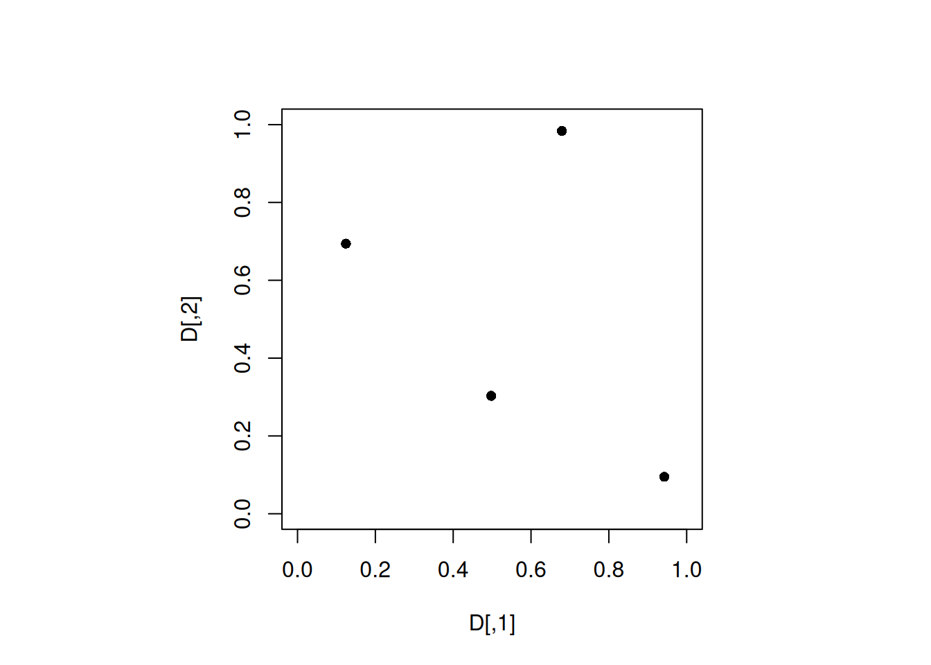
min(apply(D, 1, minimum_distance, D = D))[1] 0.4907556Note that the design has 4 distinct projections for each of the two factors.
As with maximin designs, the function maximinLHS() is an iterative algorithm that does not guarantee the global optimum. Thus, we need to run the algorithm with different seeds to find a good MaximinLHD.
min_dist <- rep(0, 20)
for(s in 1:20)
{
  set.seed(s)
  D <- maximinLHS(n = 4, k=2)
  min_dist[s] <- min(apply(D, 1, minimum_distance, D = D))
}
The seed for the best MaximinLHD is:
which.max(min_dist)[1] 6Let us plot the best MaximinLHD.
set.seed(6)
D <- maximinLHS(4, 2)
par(pty="s")
plot(D, xlim = c(0, 1), ylim = c(0, 1), pch = 16)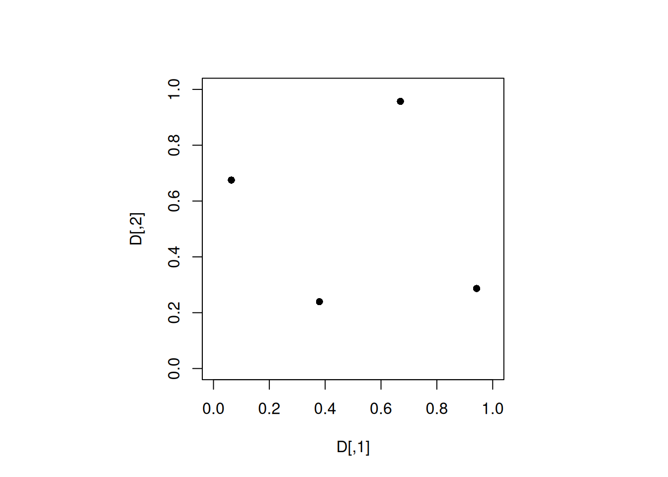
min(apply(D, 1, minimum_distance, D = D))[1] 0.5378826.2.1 MmLHD: Weakness
MaximinLHD have good projections in a single dimension, but projection properties in \(2, 3, …, p−1\) dimensions may not be good.
Let us compare the projections of a 20-run 2-dimensional design with that of a 20-run 10-dimensional design on a two-dimensional subspace.
The best 20-run MmLHD for \(p=2\) is with seed:
min_dist <- rep(0, 10000)
for(s in 1:10000)
{
  set.seed(s)
  D <- maximinLHS(n = 20, k=2)
  min_dist[s] <- min(apply(D, 1, minimum_distance, D = D))
}
which.max(min_dist)
[1] 7312The best 20-run MmLHD for \(p = 10\) is with seed:
min_dist <- rep(0, 10000)
for(s in 1:10000)
{
  set.seed(s)
  D <- maximinLHS(n = 20, k=10)
  min_dist[s] <- min(apply(D, 1, minimum_distance, D = D))
}
which.max(min_dist)
[1] 2541Let us visualize the projections of the 20 run 2-dimensional MmLHD, and the 20-run 10-dimensional MmLHD on a 2-dimensional subspace, where the subspace is the subspace of the first two predictors.
set.seed(7312)
D <- maximinLHS(20, 2)
par(mfrow = c(1,2))
par(pty="s")
plot(D, pch = 16, main = "MmLHD(n = 20, p = 2)")
set.seed(2541)
D <- maximinLHS(20, 10)
par(pty="s")
plot(D[,1:2], pch = 16, main = "MmLHD(n = 20, p = 10)")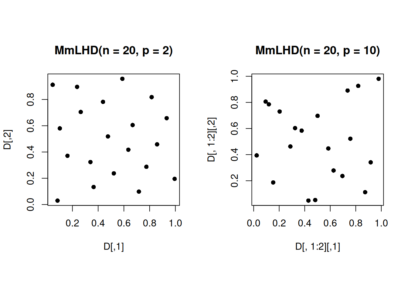
We observe that the projections of the 10-dimensional MmLHD are not as space-filling in the 2-dimensional subspace as the projections of the 2-dimensional MmLHD.
This issue motivates us to present a design that maximizes space-filling of the design projections in all multidimensional sub-spaces.
6.3 MaxProLHD & MaxPro
Let us generate a 20-run MaxProLHD and MaxPro designs in \([0, 1]^{10}\) for \(p=10\).
We will use the MaxProLHD() and MaxPro() functions of the MaxPro library
library(MaxPro)Let us find the best MaxProLHD design among 100 different MaxProLHDs. The seed that corresponds to the least MaxPro criterion is:
maxpro_criterion <- rep(0, 100)
for(s in 1:100)
{
  set.seed(s)
  Dm <- MaxProLHD(n = 20, p = 10)
  maxpro_criterion[s] <- Dm$measure
}
which.min(maxpro_criterion)
[1] 26We will use the seed to visualize the projections of a 20-run MaxProLHD and MaxPro design in 10 dimensions on a 2-dimensional subspace.
set.seed(26)
D1 <- MaxProLHD(20, 10)$Design
D2 <- MaxPro(D1)$Design
par(mfrow = c(1,2))
par(pty="s")
plot(D1[,1:2], pch = 16, main = "MaxProLHD(n = 20, p = 10)")
par(pty="s")
plot(D2[,1:2], pch = 16, main = "MaxPro(n = 20, p = 10)")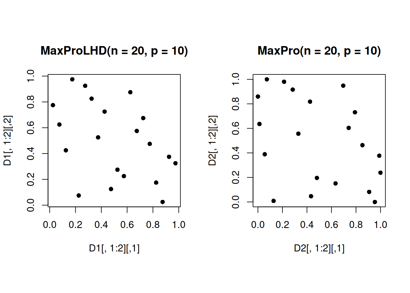
Let us compare the 2-dimensional projections of the 20-run MaximinLHD with MaxPro design.
par(mfrow = c(1,2))
par(pty="s")
plot(D[,1:2], pch = 16, main = "MmLHD(n = 20, p = 10)")
par(pty="s")
plot(D2[,1:2], pch = 16, main = "MaxPro(n = 20, p = 10)")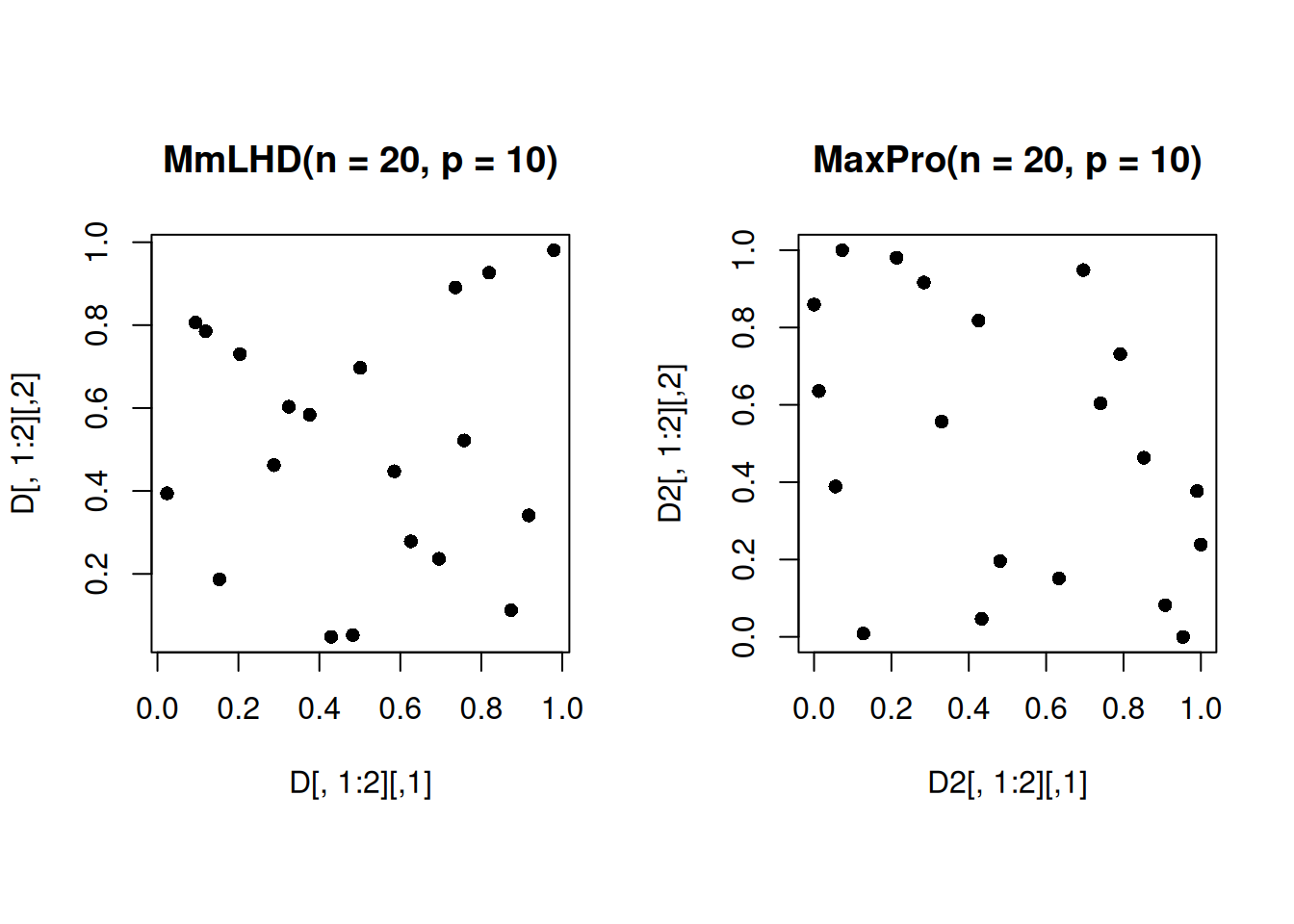
Note that the projections of the MaxPro design in the 2-dimensional subspace are more space-filling than that of the MaximinLHD, as expected.
6.4 Low descrepancy sequences
We will use the library randtoolbox to generate low-discrepancy sequences.
library(randtoolbox)Loading required package: rngWELLThis is randtoolbox. For an overview, type 'help("randtoolbox")'.6.4.1 Sobol
Let us visualize a 100-run 2-dimensional Sobol sequence.
D_sobol <- sobol(100, 2)
par(pty="s")
plot(D_sobol)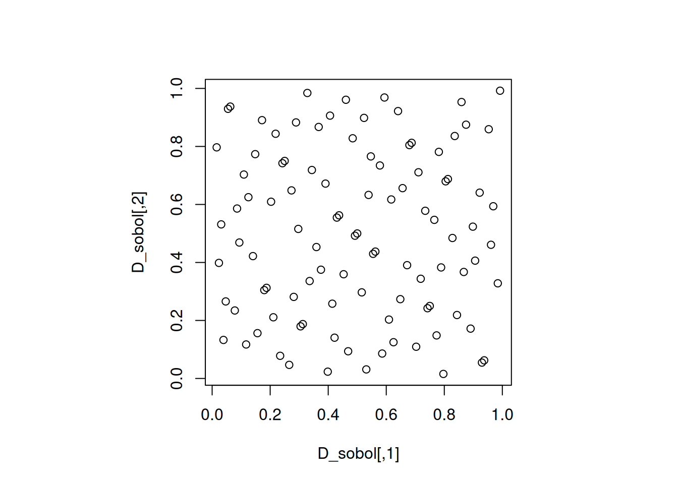
As we can see, low descrepancy sequences minimize the difference between the proportion of points in a subregion and the proportion of the volume of that subregion. However, they do not necessarily have good projections. The same is true for the Halton sequence in the next section.
6.4.2 Halton
Let us visualize a 100-run 2-dimensional Halton sequence.
D_halton <- halton(100, 2)
par(pty="s")
plot(D_halton)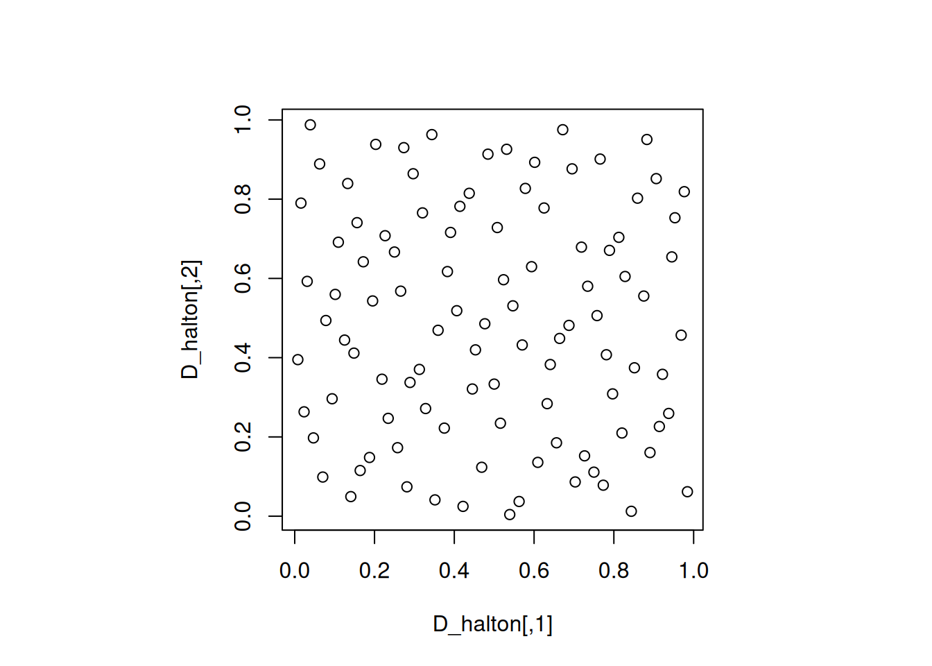
6.5 Comparison of time taken by each design
Let us compare the time taken by each design to generate a 50-run design in 50 dimensions.
n=50
time_measure <- matrix(0, 10, 6)

# Sobol
time_start <- proc.time()[3]
for(i in 1:10)
{
  D <- sobol(n, 5)
  time_measure[i,1] <- proc.time()[3] - time_start
}

# Halton
time_start <- proc.time()[3]
for(i in 1:10)
{
  D <- halton(n, 5)
  time_measure[i,2] <- proc.time()[3] - time_start
}

# Maximin
time_start <- proc.time()[3]
for(i in 1:10)
{
  D_initial <- matrix(rep(0, 5),1,5)
  D <- maximin(n = n-1, p=5, Xorig = D_initial)$Xf
  time_measure[i,3] <- proc.time()[3] - time_start
}

# MaximinLHD
time_start <- proc.time()[3]
for(i in 1:10)
{
  D <- maximinLHS(n = n, k=5)
  time_measure[i,4] <- proc.time()[3] - time_start
}

# MaxProLHD
time_start <- proc.time()[3]
for(i in 1:10)
{
  Dm <- MaxProLHD(n = n, p = 5)
  time_measure[i,5] <- proc.time()[3] - time_start
}

# MaxPro
time_start <- proc.time()[3]
for(i in 1:10)
{
  D1 <- MaxProLHD(n = n, p = 5)$Design
  d2 <- MaxPro(D1)$Design
  time_measure[i,6] <- proc.time()[3] - time_start
}
boxplot(time_measure, names = c("Sobol", "Halton", "Maximin", "MmLHD", "MProLHD",
"MaxPro"), ylab = "Time (in seconds)")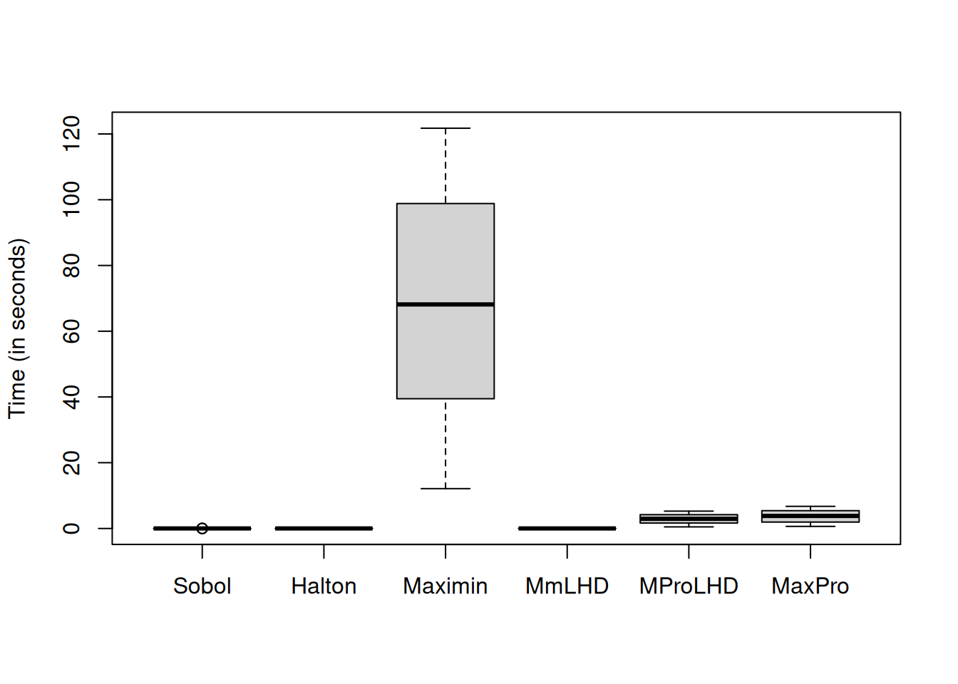
Maximin design takes the longest time as there are no constraints in the design criterion.
Let us remove the maximin design from the plot to visualize the comparison of other designs more clearly.
boxplot(time_measure[,-3], names = c("Sobol", "Halton", "MmLHD", "MProLHD",
"MaxPro"), ylab = "Time (in seconds)")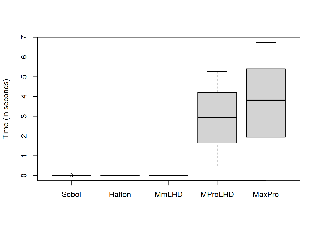
MaxProLHD and MaxPro take longer time than MmLHD as the MaxPro criterion is optimized.
Let us remove MaxProLHD and MaxPro from the plot to compare the time taken by MmLHD with low descrepancy sequences.
boxplot(time_measure[,-c(3,5:6)], names = c("Sobol", "Halton", "MmLHD"),
        ylab = "Time (in seconds)")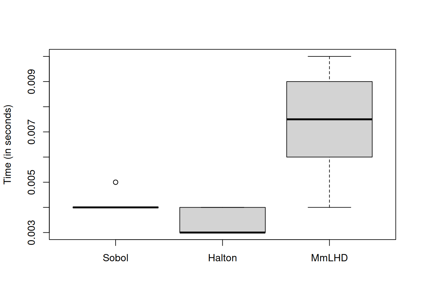
As expected, MmLHD takes more time as it includes optimization of the MmLHD criterion.